DAC Reporting in OBIEE

The purpose of this blog is to show how to consume data in the DAC repository via OBIEE reports.

What is DAC?

Oracle Business Intelligence Data Warehouse Administration Console (Oracle DAC) provides a centralized console for schema management, configuration, administration, loading, and monitoring of the Oracle Business Analytics Warehouse. The Data warehouse Application Console (DAC) is used to create and schedule Informatica ETL workflows. It manages the following data warehouse load processes:

• Dynamic generation of subject areas and execution plans
• Dynamic settings for parallelism and load balancing
• Intelligent task queue engine based on user-defined and computed scores
• Index management for ETL and query performance
• Embedded high-performance OTLP change capture techniques
• Restart from any point of failure

DAC / ETL Statistics

The metadata for ETL is stored in the DAC repository that is composed of approximately 120 tables. These tables store the ETL metadata such as tasks, task steps, execution plan details, connection details, run history, etc.

In this exercise we are only interested in the run history table - W_ETL_DEFN_RUN. This table has the ETL execution details for every Execution plan that was run through DAC (see screenshot below).

We will be walking you through the steps for creating a simple solution that will allow you to analyze the metadata in W_ETL_DEFN_RUN in OBIEE.

RPD

Below is a simple RPD model that is based on the single W_ETL_DEFN_RUN table from the DAC repository.

Reports

Using the subject area (Statistics – ETL) shown above, you can build useful reports to analyze the execution history (for each execution plan type).

1. Current month summary view with duration in minutes & hours.

2. Snapshot of run duration for each month.

Notice the failed steps in orange below.

3. Report showing Error / Status description with number of steps – Total, Failed, and Success.

4. Compare the ETL for large duration (2010 and 2011).

By adding other repository tables into your RPD you will be able to develop more sophisticated reports. You can even have error reports delivered to you with iBots whenever ETL errors occur.

How-To: Creating a Universe with the BO XI 4.0 Information Design Tool

The following describes the steps to create a universe with SAP BusinessObjects XI 4.0's new Information Design Tool.


We would like to start with a graphic displaying a systematic method to create universes in the new tool.

Figure 1: Universe Creation Flowchart for the Information Design Tool

There are a few new terms that may jump out as you are reading this, but in case you have not noticed them, let's take a minute to list those terms out:

• Connection – define how a universe connects to a relational or OLAP database. Local connections are stored as .CNX files, and secure connections are stored as .CNS files.
  
• Data Foundation – a schema that defines the relevant tables and joins from one or more relational databases. The designer enhances the data foundation with contexts, prompts, calculated columns, and other SQL definitions. The data foundation becomes the basis of one or more business layers.
  
• Business Layer – the universe under construction, and when the business layer is complete, it is compiled with the connections or connection shortcuts and data foundation, published, and deployed as a universe.
  
• Universe – the compiled file that includes all resources used in the definition of the metadata objects built in the design of the business layer.
  

Each of the items above refers to a resource that can be stored in a Project when developing in the Information Design Tool. A project is a named local workspace that contains one or more resources used to build universes. Projects can be shared so that multiple designers are able to work on the same resources.

Step 1: Open the Information Design Tool. The new interface screen will be displayed.

NOTE – All created resources will be labeled as "TestProject[resourceType]", i.e. "TestProjectConn" for Test Project Connection.

Figure 2: New Interface Screen

Step 2: Create a new Project by clicking on File->New->Project.

Figure 3: Create Project Option

A local project must exist to assign resources; otherwise an error message will be given.

Figure 4: Sample Error if no local project exists

Figure 5: New Local Project Created

Step 3: Create a new Connection. Right-click on the project you just created, or use "File->New" and choose the Relational Connection or OLAP Connection.

For the purpose of this entry, we will be creating a Relational Connection.

Figure 6: Choose a Connection

Figure 7: Define a name for Connection

Step 4: Select the proper Database Middleware driver and configure the connection. The tool comes equipped with several DB driver connections with a default installation.

Note – You must have proper privilege to the schema you are accessing. Also, an ODBC or OLE DB connection must already be established to function properly.

Figure 8: Choose the Middleware Driver

Figure 9: Connection Configuration 1

Figure 10: Connection Configuration 2

Figure 11: Connection Configuration 3

Figure 12: New Local Connection Created

A new connection should now be present and expanded in the project. This connection remains local to the project. Connections to be used in published universes will need to be published to the repository and saved as secure connections.

Step 5: Publish the connection to the repository as a secure connection. Right-click on the new local connection, or highlight the connection and choose the "File->Publish->Publish Connection to a Repository" option.

Figure 13: Publish the Connection to a Repository

Figure 14: Secure Connection Shortcut Established

Step 6: Create a new Data Foundation and configure the Data Foundation. Right-click on the project you created, or use the "File->New->Data Foundation" option.

Figure 15: Data Foundation Configuration 1

Note – there are two types of data foundations: Single-Source and Multisource-Enabled.

Single-Source

• Support a single connection.
  
• The connection can be local or secured, which means you can publish universes based on the data foundation either locally or to a repository.
  
• Recommended for the following situations: you want to work exclusively with database-specific SQL syntax, or you want to publish the universe locally and work outside of a repository.

Multisource-Enabled

• Support one or more connections.
  
• You can add connections when you create the data foundation and anytime later.
  
• Multisource-enabled data foundations only support secured connections, and universes based on this type of data foundation can only be published to a repository.
  
• Required for the following situations: you want to insert tables and joins from more than one relational data source, you want to insert tables and joins from more than one relational data source, or you want to use SQL-92 syntax and SAP BusinessObjects SQL functions.

Figure 16: Data Foundation Configuration 2

Step 7: Select the Connection to associate to the Data Foundation.

Figure 17: Data Foundation Configuration 3

Figure 18: Data Foundation Created

Step 8: Choose the Tables to Insert. You also have an option to insert Derived Tables and Views as well.

Note – Joins to objects in the Data Foundation can either be detected or manually inserted.

Figure 19: Insert Tables for Data Foundation 1

Figure 20: Insert Tables for Data Foundation 2

Figure 21: Data Foundation Created

Step 9: Create a Business Layer. Right-click on the project you created, or use the "File->New" and choose the Relational Business Layer or OLAP Business Layer. The type of business layer depends upon the connection that you used for the Data Foundation.

Figure 22: Business Layer Configuration 1

Step 10: Select the Data Foundation that you would like to use as the basis for the business layer. The tool also provides the option to automatically create classes and objects based on the Data Foundation Layer.

Figure 23: Business Layer Configuration 2

Figure 24: Business Layer Created

Step 11: Publish the Universe to the Repository. Right-click the Business Layer and choose the "Publish->To a Repository" option. This will save the Universe as a .UNX file.

Note – Ensure the Connection for the corresponding Data Foundation is a Secure Connection.

Figure 25: Publish Universe 1

Step 12: Execute a Universe Integrity Check and ensure critical errors are resolved.

Figure 26: Publish Universe 2

Step 13: Choose the Repository Folder to store the Universe.

Figure 27: Publish Universe 3

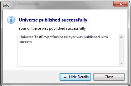
After clicking the "Finish" button, the Universe is successfully published and ready for use by the users.

Figure 28: Universe Published

You can verify that the Universe is available by logging into Interactive Analysis and creating a new document.

Figure 29: Universe Available for use in Interactive Analysis

This concludes the guide to create a Universe using the Information Design Tool. As you can see, some new terminology has been added along with a different approach to create an entire universe. We feel that the new layout and approach is tailored for multiple information designers to work on specific resources. Even though no official statement has been made by SAP BusinessObjects, we believe that the Information Design Tool will become the eventual successor to the Universe Design Tool.

Overview of Business Objects XI 4.0

SAP recently released its Business Objects Enterprise 4.0 Business Intelligence (BI) platform. The new version made updates to enhance both the end user experience and the administration of the application.

End Users

The new home page for Business Objects 4.0 is the BI Launch

pad. Formerly called InfoView, BI Launchpad welcomes users to Business Objects with a home page similar to iGoogle. Widgets displayed on the home page include My Applications, My Recently Viewed Documents, Unread Messages in My Inbox, My Recently Run Documents, and Unread Alerts. A ‘Widget’ is a user interface allowing quick access to data or an application. The BI Launchpad also features tabbed browsing.

When logging in, users have two default tabs, a home tab (previously mentioned) and a documents tab. The Documents tab gives users the old InfoView Folders view featuring Favorites and Inbox. Another advantage of tabbed browsing is the ability to have multiple reports open at once, a feature Business Objects users have wanted for awhile now. Users have the option to pin reports/documents, making them available for quick access each time the user logs into the system. Below is a screenshot of the BI Launchpad.

Another user tool modified for the Business Objects 4.0 release was WebIntelligence. WebIntelligence is also called Interactive Analysis for this release. The best feature added to the WebIntelligence tool is a raw data view available in the query panel. Users simply click a Refresh button when building their query and 15 rows of raw data are presented allowing for a quick analysis of the returned data set sample. See the screenshot below for an example of the Data Preview feature.

This allows the user to modify the query if the expected results are not shown before running a larger report. Other highlights include more chart types with additional chart features, toolbars in ribbon form similar to Office 2007, and greater consistency between the Java and Web Interfaces.

Other user tools updated with the Business Objects 4.0 release include Desktop Intelligence, Xcelsius, Life Office, Voyager, and Explorer. Desktop Intelligence is eliminated from the Business Objects Enterprise package. All Desktop Intelligence reports must be converted to either Crystal Reports or Web Intelligence reports. The report conversion tool can be used before or after the Business Objects 4.0 upgrade is performed. Xcelsius is still available but has been renamed to Dashboard Design. Live Office is incorporated within the release, allowing BI content to be more accessible throughout the Microsoft Office suite. Voyager, Business Objects’ OLAP data analysis tool, has been replaced with Advanced Analysis. Advanced Analysis highlights an enhanced task and layout panel view to improve productivity and depth of analysis for multidimensional data. SAP Business Objects Explorer is a data discovery application that allows users to retrieve answers to business questions from corporate data quickly and directly. Explorer is installed as an add-on to Business Objects Enterprise 4.0, and can be integrated with the BI Launchpad.

Administrators

Administration updates have been made throughout the Business Objects 4.0 Enterprise.

The look and feel of the Central Management Console (CMC) is similar to that of BOXI 3.0, although several features have been updated for greater user administration. Auditing has been updated throughout the release. The CMC Auditing feature allows administrators to modify what is being audited. Monitoring is now available through the CMC. Monitoring allows administrators to verify all components of the system are functioning properly. Response times can be viewed and CMS performance can be evaluated within the Monitoring feature. See the screenshot below for the Monitoring interface.

Universe design received an update in the 4.0 release with a new tool called the Information Design tool. The highlights of the tool include the ability to create multisource universes, dimensional universes that support OLAP dimensions and hierarchies, and easier management of repository resources. Each universe will now consist of three files (or layers), a connection layer, a data foundation, and a business layer. The connection layer defines the connections used for universe development. The data foundation layer defines the schemas being used for a relational universe. The business layer is the universe created based on your data foundation. Resources can be shared, allowing connections and data foundations to help create multiple business layers (or universes). Below is a screenshot showing the Information Design Tool. The upper left shows the project with the different layers created. The bottom left shows the shared repository resources. The right side is similar to previous versions of Business Objects Designer.

Import Wizard has been replaced by two separate tools, the Upgrade Management tool and the Lifecycle Management Console. The Upgrade Management tool allows for direct upgrades from Business Objects XI R2 SP2 or later. The new easy to use interface allows upgrades to go more smoothly. The Lifecycle Management Console is a web-based tool which gives administrators a way to handle version management. Rollback and promotion of objects is available among different platforms if the same version of Business Objects is being used.

Getting to 4.0

Business Objects 4.0 is a complete new install, an upgrade option is not available. To migrate over specific application resources (Universes, CMS data, etc.), older versions of Business Objects (5.x, 6.x) must be upgraded to Business Objects XI R2 or later first. The deployment of 4.0 has also been simplified through the use of a single WAR file for web application deployment. Business Objects servers and web application tier can only be installed and run on 64-bit operating systems.

The Art of Identifying Meaningful BI Requirements

We have seen time and time again that the success of DW/BI implementations is dependent on the ability to identify BI requirements that have a measurable impact on the organization’s business decision making process (see our blog article “You just need three letters: WHY?”). However, identifying such requirements is a not a trivial process. A repeatable process is needed that is designed to keep the focus on the client’s business when developing business requirements for a DW/BI implementation. The following sections describe an overall approach with suggested techniques that we have used successfully.

Macro Level Understanding of Business

It is important to understand how your organization operates: how the business runs in order to make the best use of your BI capability. When you understand the key business processes and key business objectives, you can begin to drill down into more details that will provide not only reporting requirements, but also the data elements that are required to support those requirements.

Business Processes/Objectives

By understanding the business at a high level, you can begin to understand the business processes that support the organization. We need to understand what the key business processes are, then we need to understand how they work. We also strive to understand the core business objectives. Ultimately, all decisions that the customers make should support one or more business objectives. Once we identify business decisions, we can more easily identify detailed business questions and related data elements. The business questions will lead directly to specific reports or sets of reports. The data elements will support those reports and potential ad hoc analysis needs.

How to Implement

We can use the following tools and techniques to implement this requirements process. Background Research provides initial information about the nature of the business and its processes. It can help provide a preliminary list of decision centers, activities, and major decisions that are part of the organization you are focused on.

Structured Interviews should be used to build on the initial research you have gained. Seek out those who are knowledgeable of the organizational business processes. Through the interview process, the interviewer can gain information about problems, decisions, or critical success factors that are part of the running of the business. This high-level information can be used as a starting point in gathering more detailed requirements necessary for building a decision support system. Ask questions that lead the interviewee to indirectly identify information that supports decision-making. One approach is to ask the interviewee to identify the major business drivers that they are responsible for. Once these drivers are identified, ask them to identify the major decisions that they need to make to support those business drivers and one or more questions that they ask in the process of making each decision. Another approach is to ask your customer to identify the critical success factors they are responsible for. The individual should then be asked to identify for each critical success factor the information they need to ensure that the critical success factor is under control.

Joint Application Design (JAD) is a communal effort to further refine and agree on the hierarchy of business needs. When individuals are interviewed alone, they tend to respond to questions more or less in a vacuum; without the context of others’ views on how information is used. They also may have difficulty identifying a comprehensive set of answers to each question they are asked. A JAD session helps to elicit greater “thinking” by the participants as they hear other ideas and perspectives. A JAD session helps to bring out more decisions and business questions as more approaches are identified. The result: a more complete set of requirements upon which to build a BI system. The JAD session will be most successful if the right people are present. Individuals who have a solid understanding of each of the business processes to be covered, have the authority to make design decisions, and communicate well, should participate. The facilitator should be knowledgeable in BI system design as well as the business being supported. A JAD session should be held only after you have identified a baseline of business drivers, business decisions, and business questions based on information from the initial set of structured interviews and research.

Prototyping is a technique used after initial requirements have been established. Based on the information gathered from interviews and JAD sessions, you can develop an initial reporting database with limited BI reports. This gives you an opportunity to demonstrate the information and functionality of the reports to end users early in the development process. The feedback you received will help you to fine-tune your product early in the process so that the delivered product more closely meets your customer’s needs.

The figure below summarizes how a top-down approach will help to derive both reporting requirements as well as supporting data elements. For each business objective, there may be several business processes and decisions to support that objective. Each process and decision will involve business questions that need to be answered to support the process or decision. A business question may drive a specific report requirement. Meanwhile, each business question will require multiple data elements. By going through this process, you not only identify business-driven requirements for your BI system; you also keep the customer more heavily involved by forcing them to think critically about how their day-to-day decisions help drive the overall business. We have found these techniques to be successful using them in different combinations based on our client situation. How have these techniques worked for you? What other methods have you found valuable in driving requirements for your reporting initiatives?

Modeling Multiple Helper Tables in OBIEE

Problem: Dimensional modeling is the preferred method of organizing data in OBIEE but at times the standard configuration for a dimensional star does not represent the way data is collected in the source system.

Traditionally, a star schema has a single fact table with many dimensions. The dimensions are related to many fact records in a one-to-many relationship to the fact. However, sometimes the relationship of the data is many-to-many. An example for this comes from the healthcare industry where one doctor visit record can be associated with multiple diagnosis codes.

We encountered such relationships at a recent project. One of the source systems at this client captured incident data. A traditional star schema did not meet our client’s requirements because this source system collected key measures at an incident grain but there was a need to analyze these measures at a grain below the level at which they were created. The incident data was organized into a six level hierarchy, each of which with a one-to-many relationship to the level below. All the important KPI’s were captured at the incident level. As can be seen in the hierarchy diagram below, an incident is the summary level (top level) of data collected.

We had to create reports at a detail level called “cause of incident” for damages or injuries captured in aggregate at the incident level. The challenge was to attribute all damages in an incident to each cause without double counting damages or injures at the grain being reported.

First, we created Incident, Shipper, Product, Container, and Cause dimensions. Next we created an incident fact table that held all appropriate measures. We then created bridge-tables for each dimension with a many-to-many relationship.

Unfortunately, bridge-tables require a weighting factor. Since the measures existed in the source system only at the summary level, the weighting factor would not correctly attribute fatalities to each detail level item. For example, an incident with 2 fatalities occurred. The incident was attributed to have been caused by an accident and fire. When counting the number of deaths because of fire the business rule is to count 2 for fire not 1 as a weighting factor of .5 would do.

So we decided to trick OBIEE. The picture below shows the central fact with many helper tables that are 1:M from the fact.

However, by leaving the join as a 1:M OBIEE treats the helpers as separate facts. The performance is awful and it does not aggregate correctly. So we changed the relationship to 1:1 and it worked. Because it is an inner join the SQL sent to the database returns the correct number of rows and OBIEE still think the fact is a fact.

The downside is that grand totaling does not work correctly, which did not cause a problem for our requirements, though. If your client’s business rule is to attribute summary level measures equally across the details then a bridge table will work with the appropriate weights. If you need to have multiple many-to-many details using un-weighted summary level measures this solution will work. In summary, this method may not work for every project but for some business requirements it will make a challenging scenario work.

Please contact us if you have any questions.

Identifying Source System Data Changes for Incremental ETL Processes

Problem: When designing incremental ETL processes, ETL Architects face the challenge of identifying algorithms to identify data changes in the source system between ETL runs. Some of the options that might be available are (from the best case scenario to the worst):

1. Database Log Readers: This approach utilizes an ETL tool that is capable of reading the source database log files to identify inserted and updated records. For example, Informatica Power Center supports this through its Change Data Capture (CDC) functionality. However, source system owners may not be willing to grant read access to the database logs or an ETL tool that supports this functionality may not be available.
2. Timestamp columns in the source database: If the source system maintains an insert and update timestamp column for each table of interest, then the ETL process can utilize these columns to identify source system changes since the last ETL execution timestamp. Chances are, however, that the source system does not provide that functionality.
3. Triggers to populate log tables: This is by far the worst option since it adds a significant resource utilization burden to the source system. In this case, triggers are created for all tables of interest. The purpose of these triggers is to capture all insert/updates/deletes into log tables. The ETL process then reads the data changes from the log tables and removes all records that it has successfully processed. Again, source system owners will most likely be very hesitant to support this approach.

What to do if none of these options are available?



Solution: We propose the following checksum based approach. In this blog, we will utilize SQL Server’s CHECK_SUM algorithm; however, Oracle’s ORA_HASH can be used in a similar fashion.

This approach requires that the entire source table (only columns and rows of interest, of course) be loaded into a staging table. During the staging load, the ETL process will assign a checksum value to each record. For example, when loading data from SOURCE_TABLE_A into STAGING_TABLE_A, the SQL would look something like this:

insert into staging_table_a ( col1, col2, cold3, business_key, check_sum)
select col1, col2, cold3, business_key, check_sum(col1,col2,cold3,business_key)
from source_table_a

Let us further assume that business_key is the primary key of the source system record. In other words, business_key uniquely identifies a record in the source system.

Both business_key and check_sum must be stored in their corresponding dimension tables. In our example, the dimension table for source_table_a would include a surrogate dimension key (dim_key), business_key, and check_sum as shown below.
For performance optimization reasons, we recommend to create a composite index on business_key and check_sum.

In order to identify new records that were inserted into the source system since the last ETL run, we have to find all business_keys in the staging table that have no corresponding business_key in the dimension table. The SQL code would look something like this:

select s.* from staging_table_a s
Where not exists (select * from dimension_table_a d
where d.business_key = s.business_key)

To identify updated records since the last ETL run, we have to find all records in the staging table that have a matching business_key in the dimension table with a different check_sum value. Here is the SQL code for this:

select s.*
from staging_table_a s
inner join dimension_table_a d on
d.business_key = s.business_key and
d.check_sum <> s.check_sum

In all cases, the joins against the dimension table will be based on index lookups because we have a composite index on business_key and check_sum. Therefore, identifying new or updated records is quite efficient. The drawback of this solution is the necessity to perform a full data load into the staging area, which may not be feasible for large source systems.

One of the major benefits of this approach is its immunity against getting out-of-sync with the source system (due to aborted or failed ETL processes). No matter at what point the previous ETL process has failed, this approach will always correctly identify source system changes and re-sync without any additional human intervention.

In summary, the check_sum approach may be a feasible alternative for environments that have no other means for identifying data changes in the source system.

Please contact us if you have any questions.